Bloom Filters Demystified: How They Work and Why They’re Useful
Learn how Bloom filters work, their applications, and why they're useful in data structures and algorithms.
#Bloom Filters: A Comprehensive Guide
##Table of Contents
- Introduction
- The Problem Space
- What Is a Bloom Filter?
- How It Works
- Mathematical Foundation
- Bloom Filters vs. Other Data Structures
- Kirsch-Mitzenmacher Hashing
- Implementation: Code Block by Block
- Limitations
- Real-World Applications
##Introduction
A Bloom filter is a space-efficient, probabilistic data structure used to test whether an element is a member of a set. Conceived by Burton Howard Bloom in 1970, it was designed for scenarios where memory is scarce and exact answers are not strictly necessary. The trade-off is elegant: a Bloom filter can tell you with certainty that an element is not in the set, or that it is probably in the set. False positives are possible, but false negatives are not.
"Space/Time Trade-offs in Hash Coding with Allowable Errors" — Burton H. Bloom, Communications of the ACM, July 1970.
Bloom filters have since become a staple in systems programming, networking, databases, and web infrastructure because they can represent huge sets using only a few bits per element.
##The Problem Space
Imagine you need to answer a simple question: "Have I seen this URL before?"
A naïve approach would store every URL in a std::set or std::unordered_set in memory. For millions or billions of URLs, this requires petabytes of RAM—impractical for client-side devices, network routers, or high-performance caches.
Conventional error-free hashing also falls short. To guarantee zero false positives, you need one full hash table slot per element, plus overhead for the hash table structure itself. When the dataset exceeds available memory, you are forced to make a choice:
- Store everything exactly → run out of memory.
- Store nothing → miss every query.
- Store a compact summary → accept a small chance of error.
Bloom filters choose option 3. They compress a set into a fixed-size bit array, trading a configurable amount of accuracy for dramatic space savings.
##What Is a Bloom Filter?
A Bloom filter consists of two components:
- A bit array of
mbits, all initialized to 0. kindependent hash functions, each mapping an input element to a bit index in[0, m).
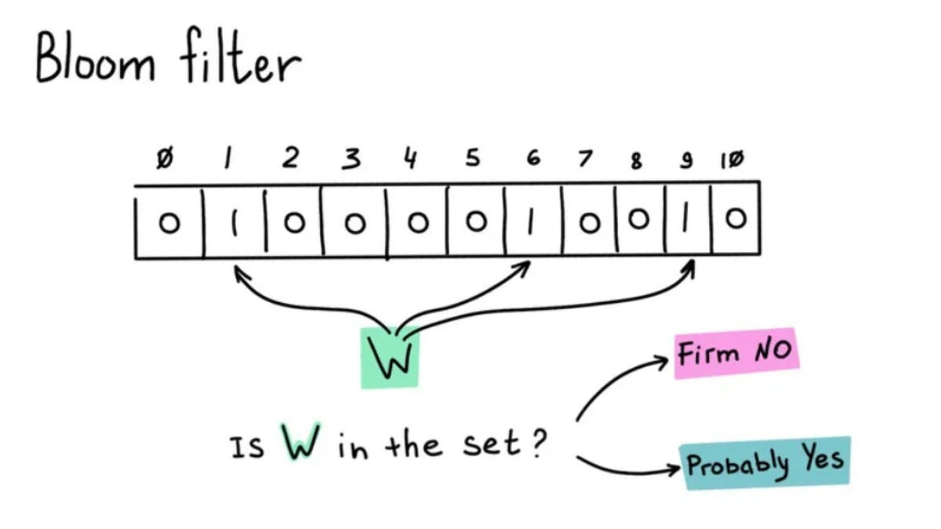
When an element is inserted, each of the k hash functions produces an index, and the corresponding bits are set to 1.
When an element is queried, the same k hash functions are applied. If every corresponding bit is 1, the filter reports "possibly in set". If any bit is 0, it reports "definitely not in set".
Because bits can be shared among many elements, the filter never needs to store the element itself. This is what makes it so compact.
##How It Works
###The Bit Array
At the core of every Bloom filter is a simple array of bits. In this implementation, bits are packed into 64-bit words (uint64_t) for cache-friendly access. An array of m bits only requires m / 64 machine words.
###Hash Functions
The filter uses k hash functions to transform an input key into k distinct positions in the bit array. The key property is that these positions should be uniformly distributed and effectively independent.
###Insert
To insert a key:
- Compute
khash values. - For each hash value
h, setbit[h] = 1.
###Query / Membership Test
To check if a key is present:
- Compute the same
khash values. - For each hash value
h, readbit[h]. - If any read returns 0 → the key is definitely not in the set.
- If all reads return 1 → the key is probably in the set.
###False Positives Explained
A false positive occurs when a key not in the set hashes to k positions that were all previously set to 1 by other inserted keys. Because bits are shared, collisions are inevitable. The false positive probability is controlled by the ratio of k (hash functions) to m (bit array size) and the number of inserted elements n.
Crucially, false negatives are impossible. If a key was inserted, all its k bits were set to 1. Nothing ever resets a bit to 0 (in the standard Bloom filter), so a query for an inserted key will always find all k bits set.
##Mathematical Foundation
Bloom filters are governed by three key equations. Given:
n— expected number of elements to insertp— desired false positive rate (e.g., 0.01 for 1%)m— number of bits in the arrayk— number of hash functions
###Optimal Bit Count
To achieve a false positive rate p with n elements, the optimal number of bits is:
This minimizes memory while meeting the accuracy target. Note that m does not depend on the size of the keys themselves—only on n and p.
###Optimal Hash Count
Given n and m, the optimal number of hash functions is:
This balances the probability of a bit remaining 0 against the probability of over-hashing (which increases false positives).
###False Positive Probability
After inserting n elements, the probability that a specific bit is still 0 is:
A false positive occurs when all k queried bits are 1, so:
At the optimal k, this simplifies to approximately:
In practice, fewer than 10 bits per element are required for a 1% false positive rate, independent of the dataset size.
##Bloom Filters vs. Other Data Structures
| Data Structure | Lookup | Insert | Delete | Memory | False Positives |
|---|---|---|---|---|---|
| Bloom Filter | O(k) | O(k) | No | O(m) ≈ O(n) bits | Yes (configurable) |
| Hash Set | O(1) | O(1) | Yes | O(n) × key size | No |
| Sorted Array | O(log n) | O(n) | Yes | O(n) × key size | No |
| Trie | O(len(key)) | O(len(key)) | Yes | O(n) × len(key) | No |
###Vs. Hash Set
A hash set stores each element exactly, providing zero false positives and supporting deletion. However, it must store the full key for every element. For strings or large keys, the overhead is significant—often 10× to 100× larger than a Bloom filter for the same number of items. A Bloom filter is preferable when:
- Keys are large (URLs, email addresses, IP addresses).
- Memory is the primary constraint.
- False positives are acceptable and can be handled by a secondary exact check.
###Vs. Sorted Array / Binary Search
A sorted array allows binary search (O(log n)) and is memory-compact, but insertion is expensive (O(n) due to shifting). It also requires storing the full keys. Bloom filters are superior when writes are frequent and reads must be O(1)-like.
###Vs. Tries (Prefix Trees)
Tries excel at prefix queries and ordered traversal, but they carry heavy pointer overhead and memory fragmentation. A Bloom filter provides no prefix guarantees, but it is far more compact and cache-friendly for simple membership testing.
###When to Choose a Bloom Filter
Use a Bloom filter when:
- You need to test set membership for millions/billions of items.
- Memory is limited (e.g., embedded systems, network devices).
- Most queries are expected to be negative (non-members).
- You can tolerate a small false positive rate.
- You do not need to delete items (or can use a counting variant).
Avoid a Bloom filter when:
- False positives are unacceptable (e.g., financial transaction validation).
- You need to enumerate or iterate over the set.
- Deletions are frequent and required.
##Kirsch-Mitzenmacher Hashing
Computing k independent hash functions for every operation can be expensive. In 2006, Kirsch and Mitzenmacher proposed a clever optimization: two hash functions are sufficient.
Instead of computing h₁(x), h₂(x), ..., hₖ(x) independently, compute only:
for i = 0, 1, ..., k-1.
This linear combination of two base hashes produces indices that are sufficiently independent for practical Bloom filter use, while halving (or more) the hashing computation. The technique is described in the paper "Less Hashing, Same Performance: Building a Better Bloom Filter" (Kirsch & Mitzenmacher, ESA 2006).
##Implementation: Code Block by Block
The following walkthrough examines each part of the Bloom filter implementation in this codebase.
###BitArray — The Foundation
The Bloom filter relies on a raw bit array. Because individual bits cannot be addressed directly in C++, they are packed into uint64_t words.
include/BitArray.hpp
#ifndef BIT_ARRAY_HPP
#define BIT_ARRAY_HPP

#include "Globals.hpp"

class BitArray {
   public:
	BitArray(size_t bits);

	void set(size_t index);

	bool get(size_t index) const;

	size_t size() const { return num_bits; }

   private:
	std::vector<uint64_t> data;
	size_t num_bits;
};
#endif	// !BIT_ARRAY_HPP
The interface is minimal:
set(index)— flips a bit to 1.get(index)— reads a bit.size()— returns the total number of bits.
src/BitArray.cpp
#include "BitArray.hpp"

#include <cassert>
#include <cstddef>
#include <cstdint>
#include <vector>

BitArray::BitArray(size_t bits)
	: data((bits + 63) / 64, 0), num_bits(bits) {}

void BitArray::set(size_t index) {
	assert(index < num_bits);
	data[index / 64] |= (1ULL << (index % 64));
}

bool BitArray::get(size_t index) const {
	assert(index < num_bits);
	return (data[index / 64] >> (index % 64)) & 1ULL;
}
Line-by-line breakdown:
BitArray::BitArray(size_t bits)
	: data((bits + 63) / 64, 0), num_bits(bits) {}
The constructor allocates (bits + 63) / 64 64-bit words. The +63 ensures we round up to the next whole word, so even a single bit gets one full uint64_t backing it. Both the vector and num_bits are initialized in the member initializer list.
void BitArray::set(size_t index) {
	assert(index < num_bits);
	data[index / 64] |= (1ULL << (index % 64));
}
set computes which word contains the bit (index / 64) and which position within that word (index % 64). It then ORs a mask with a single 1-bit shifted into position. The assert guards against out-of-bounds access in debug builds.
bool BitArray::get(size_t index) const {
	assert(index < num_bits);
	return (data[index / 64] >> (index % 64)) & 1ULL;
}
get performs the inverse: shift the target bit to the least-significant position, then mask with 1ULL to extract a 0 or 1.
###Globals.hpp — Shared Includes
include/Globals.hpp
#ifndef GLOBALS_HPP
#define GLOBALS_HPP

#include <cstddef>
#include <cstdint>
#include <cstdlib>
#include <string>
#include <vector>

#endif	// !GLOBALS_HPP
This header centralizes common standard-library includes used across the project: cstddef/cstdint for fixed-width types, cstdlib for general utilities, string for keys, and vector for dynamic storage.
###BloomFilter.hpp — Public Interface
include/BloomFilter.hpp
#ifndef BLOOM_FILTER_HPP
#define BLOOM_FILTER_HPP

#include "BitArray.hpp"
#include "Globals.hpp"

class BloomFilter {
   public:
	/// Construct a Bloom filter optimized for @p expected_elements
	/// with the given @p false_positive_rate (0 < p < 1).
	BloomFilter(size_t expected_elements, double false_positive_rate = 0.01);

	void insert(const std::string& key);

	bool contains(const std::string& key) const;

	/// Number of bits in the underlying bit array.
	size_t bit_count() const { return bits.size(); }

	/// Number of hash functions used.
	size_t hash_count() const { return num_hashes; }

   private:
	BitArray bits;
	size_t num_hashes;

	/// Compute the i-th hash index for @p key in [0, bit_count()).
	size_t hash(const std::string& key, size_t i) const;
};

#endif	// !BLOOM_FILTER_HPP
The class exposes three operations:
- Constructor — computes optimal
mandkfromexpected_elementsandfalse_positive_rate. insert— adds a key to the filter.contains— tests membership.
It also exposes two inspectors (bit_count, hash_count) so callers can inspect the computed parameters. The private hash method implements the Kirsch-Mitzenmacher scheme.
###BloomFilter.cpp — Optimal Sizing
src/BloomFilter.cpp
#include "BloomFilter.hpp"

#include <cmath>
#include <cstddef>
#include <functional>
#include <string>

#include "BitArray.hpp"
#include "Globals.hpp"

// ---- optimal-size helpers (file-static) ----

static size_t optimal_bit_count(size_t n, double p) {
	// m = -n * ln(p) / (ln(2)^2)
	double m = -static_cast<double>(n) * std::log(p) / (std::log(2.0) * std::log(2.0));
	return static_cast<size_t>(std::ceil(m));
}

static size_t optimal_hash_count(size_t n, size_t m) {
	// k = (m/n) * ln(2)
	double k = (static_cast<double>(m) / static_cast<double>(n)) * std::log(2.0);
	size_t kh = static_cast<size_t>(std::ceil(k));
	return (kh < 1) ? 1 : kh;
}
Line-by-line breakdown:
static size_t optimal_bit_count(size_t n, double p) {
	// m = -n * ln(p) / (ln(2)^2)
	double m = -static_cast<double>(n) * std::log(p) / (std::log(2.0) * std::log(2.0));
	return static_cast<size_t>(std::ceil(m));
}
This implements the optimal bit-count formula. n is the expected number of elements; p is the target false positive rate. std::ceil rounds up because we cannot allocate a fractional bit. The result is a size_t suitable for constructing the BitArray.
static size_t optimal_hash_count(size_t n, size_t m) {
	// k = (m/n) * ln(2)
	double k = (static_cast<double>(m) / static_cast<double>(n)) * std::log(2.0);
	size_t kh = static_cast<size_t>(std::ceil(k));
	return (kh < 1) ? 1 : kh;
}
This implements the optimal hash-count formula. n is the expected element count; m is the previously computed bit count. The guard (kh < 1) ? 1 : kh ensures at least one hash function is used, even for tiny filters where the formula might yield k < 1.
###BloomFilter.cpp — Insert
BloomFilter::BloomFilter(size_t expected_elements, double false_positive_rate)
	: bits(optimal_bit_count(expected_elements, false_positive_rate)),
	  num_hashes(optimal_hash_count(expected_elements, bits.size())) {}

void BloomFilter::insert(const std::string& key) {
	for (size_t i = 0; i < num_hashes; ++i) {
		bits.set(hash(key, i));
	}
}
The constructor chains the two helper functions: it first computes the optimal bit array size, then uses that size to compute the optimal number of hash functions. The insert loop iterates k times, computing a unique bit position for each i and setting it.
###BloomFilter.cpp — Contains
bool BloomFilter::contains(const std::string& key) const {
	for (size_t i = 0; i < num_hashes; ++i) {
		if (!bits.get(hash(key, i))) {
			return false;
		}
	}
	return true;
}
The query short-circuits on the first 0 bit it encounters. This is the key optimization: a single zero bit is sufficient to prove non-membership, so we rarely need to check all k bits.
###BloomFilter.cpp — The Hash Function
size_t BloomFilter::hash(const std::string& key, size_t i) const {
	// Two independent base hashes using the Kirsch-Mitzenmacker technique
	size_t h1 = std::hash<std::string>{}(key);
	size_t h2 = std::hash<std::string>{}(key + '\x01');

	if (h2 == 0) h2 = 1;  // ensure non-zero for the linear combination

	size_t m = bits.size();
	return (h1 + i * h2) % m;
}
Line-by-line breakdown:
size_t h1 = std::hash<std::string>{}(key);
The first base hash uses the standard C++ std::hash on the raw key.
size_t h2 = std::hash<std::string>{}(key + '\x01');
The second base hash is computed on key + '\x01'. Appending a sentinel byte ensures the second hash input is different from the first, producing a statistically independent second hash value without requiring a second hash algorithm.
if (h2 == 0) h2 = 1;
If h2 happens to be 0 (unlikely but possible), the linear combination h1 + i * h2 would reduce to h1 for all i, collapsing all k buckets into one. This guard prevents that pathological case by bumping a zero h2 to 1.
size_t m = bits.size();
return (h1 + i * h2) % m;
The final formula gᵢ(x) = (h₁ + i·h₂) mod m generates k distinct indices from two hashes. Because h2 is non-zero, each i produces a different offset, and the modulo folds the result into the valid bit-array range.
###main.cpp — Using the Filter
main.cpp
#include <cstddef>
#include <iostream>
#include <string>

#include "BloomFilter.hpp"
#include "Globals.hpp"

int main(int argc, char* argv[]) {
    // Create a Bloom filter for 100 elements with 1% false positive rate
    BloomFilter bf(100, 0.01);

    std::cout << "Bloom filter created:" << std::endl;
    std::cout << "  bits:      " << bf.bit_count() << std::endl;
    std::cout << "  hashes:    " << bf.hash_count() << std::endl;
    std::cout << std::endl;

    // Insert some elements
    bf.insert("apple");
    bf.insert("banana");
    bf.insert("cherry");
    bf.insert("dragonfruit");
    bf.insert("elderberry");

    std::cout << "Inserted: apple, banana, cherry, dragonfruit, elderberry"
              << std::endl;
    std::cout << std::endl;

    // Query inserted elements (should always return true)
    std::cout << "--- Membership queries (should all be 1) ---" << std::endl;
    std::cout << "apple:       " << bf.contains("apple") << std::endl;
    std::cout << "banana:      " << bf.contains("banana") << std::endl;
    std::cout << "cherry:      " << bf.contains("cherry") << std::endl;
    std::cout << "dragonfruit: " << bf.contains("dragonfruit") << std::endl;
    std::cout << "elderberry:  " << bf.contains("elderberry") << std::endl;
    std::cout << std::endl;

    // Query elements that were NOT inserted (mostly 0, occasional false positive)
    std::cout << "--- Non-membership queries (should mostly be 0) ---"
              << std::endl;
    std::cout << "fig:         " << bf.contains("fig") << std::endl;
    std::cout << "grape:       " << bf.contains("grape") << std::endl;
    std::cout << "honeydew:    " << bf.contains("honeydew") << std::endl;
    std::cout << "kiwi:        " << bf.contains("kiwi") << std::endl;
    std::cout << "lemon:       " << bf.contains("lemon") << std::endl;

    return 0;
}
The driver demonstrates the core contract:
- Construct a filter for 100 elements at 1% false positive rate.
- Print the auto-computed parameters (
bit_count,hash_count). - Insert five known elements.
- Query inserted elements—results should all be
1(true negatives are impossible). - Query non-inserted elements—results should mostly be
0, with occasional1s representing false positives.
Running the binary shows the filter in action:
$ ./build/bin/bloom_filter
Bloom filter created:
  bits:      959
  hashes:    7

Inserted: apple, banana, cherry, dragonfruit, elderberry

--- Membership queries (should all be 1) ---
apple:       1
banana:      1
cherry:      1
dragonfruit: 1
elderberry:  1

--- Non-membership queries (should mostly be 0) ---
fig:         0
grape:       0
honeydew:    0
kiwi:        0
lemon:       0
##Limitations
Standard Bloom filters have well-known constraints:
-
No deletions. Unsetting a bit could corrupt membership for other elements that share that bit. Variants like Counting Bloom Filters use multi-bit counters instead of single bits to support deletion, at the cost of higher memory usage.
-
False positives grow with load. As more elements are inserted, more bits become 1, and the false positive rate approaches 100%. The formulas assume a target
n; exceeding it degrades accuracy. -
No enumeration. Because the filter stores only hashed bit patterns, you cannot list the elements that were inserted.
-
No reverse lookup. Given a bit pattern, you cannot determine which key produced it.
##Real-World Applications
Bloom filters appear in production systems where memory, latency, and approximate answers collide.
- Web Caches: Browsers and proxies use Bloom filters to quickly determine if a resource is likely cached, avoiding expensive round-trips.
- Databases: Google Bigtable, Apache Cassandra, and PostgreSQL use Bloom filters to skip disk reads for keys that definitely do not exist in a file or SSTable.
- Spell Checkers: A dictionary of valid words is stored in a Bloom filter. Misspelled words are caught immediately; valid words pass through to a secondary checker.
- Network Routers: Routers use Bloom filters to detect malicious traffic or duplicate packets without keeping full flow state.
- Blockchain: Bitcoin nodes use Bloom filters to receive relevant transactions without revealing their full wallet addresses (privacy-preserving SPV clients).
- AdTech: Ad servers use Bloom filters to avoid showing the same ad to a user who has already seen it, without storing billions of user-view histories.
##Conclusion
Bloom filters remain one of the most elegant solutions in computer science: a few lines of mathematics and bit manipulation yield a data structure that scales to billions of elements in kilobytes of memory. By understanding the trade-offs—accepting false positives to reject false negatives—engineers can build systems that are faster, leaner, and surprisingly accurate.
The implementation in this repository demonstrates the classic design: an optimal-size bit array, the Kirsch-Mitzenmacker double-hashing optimization, and a clean C++17 interface. Whether you are building a spell checker, a database index, or a network filter, the Bloom filter is a tool worth having in your arsenal.